"A combination of noise and bilateral filters achieve supralinear and scalable adversarial robustness in CNNs."
SUMMARY
Adversarial perturbations can make convolutional neural networks fail even when the input changes are nearly invisible to humans. In this work, we study a simple defense strategy based on combining noise with bilateral filtering, and show that this combination can produce scalable gains in adversarial robustness.
1 - The intuition
An adversarial attack on an image $x$ is a perturbation vector $a_x$ small enough to be invisible to a human, yet large enough to push $x$ across the neural network's decision boundary. Formally, we require $\|a_x\| \leq r$, which defines an adversarial sphere of radius $r$ around the image. To measure how vulnerable a classifier is at a given image, we define the adversarial volume, \begin{equation} V_a(x) = \int_{z \in \mathbf{B}(x,r)} \mathbf{1}\!\left[f(z) \neq h(z) = f(x)\right] dz, \end{equation} where $\mathbf{B}(x,r)$ is the ball of radius $r$ around $x$, $f(\cdot)$ is the neural network, and $h(\cdot)$ is the true human classification. Intuitively, $V_a(x)$ measures the volume of attack-accessible space around an image that the network misclassifies. It is the central quantity in our analysis: fixing $V_a(x)$ lets us directly compare what different defenses do and do not cover.
Filters. We model a filter as an idealized denoising function $\varphi: \mathcal{X} \rightarrow \mathcal{X}$ that leaves clean images unchanged and pushes any perturbation back toward the image manifold. The worst-case attack against a filter is a thin cylinder that enters the adversarial sphere and sneaks as close to the image as possible---the filter cannot cancel it because it lies too close to the image manifold. More precisely, for a fixed $V_a(x)$, a successful attack can exist when \begin{equation} V_a(x) > r\!\left(1 - \lambda_{\varphi}^{\min}\right) S_{D-1}\!\left(c^{-1/2}\right), \end{equation} where $\lambda_{\varphi}^{\min}$ is the minimum eigenvalue of the Jacobian of $\varphi$ (how much it contracts the worst-case direction), and $S_{D-1}(c^{-1/2})$ is the surface area of a $(D{-}1)$-dimensional sphere with curvature $c$. Even when such an attack exists, the effective adversarial volume is reduced by a factor proportional to $|J_\varphi|$. In short: filters work well against attacks that live far from the image manifold, near the outer edge of the adversarial sphere.
Noise. Adding Gaussian noise with variance $\sigma^2$ to a perturbed image moves it in a random direction, disrupting adversarial attacks whenever the misclassified region is small. The worst case for noise is therefore the opposite of the worst case for filters: a large, compact adversarial region clustered around the attack point. Formally, the probability of an attack succeeding under noise is bounded by \begin{equation} \Pr\!\left[x + a_x + \varepsilon \in A\right] \leq 1 - 2\,\mathrm{erf}\!\left(-\frac{\rho_D(V_a(x))}{\sigma}\right), \end{equation} where $\rho_D(V_a(x))$ is the radius of a $D$-dimensional sphere with volume $V_a(x)$. The bound shows that noise is effective when the adversarial volume is small and spread thin (filament-shaped attacks), and ineffective when the adversarial region is large and compact. In short: noise works well against thin, filament-like attacks, but fails when the adversarial region forms a large sphere.
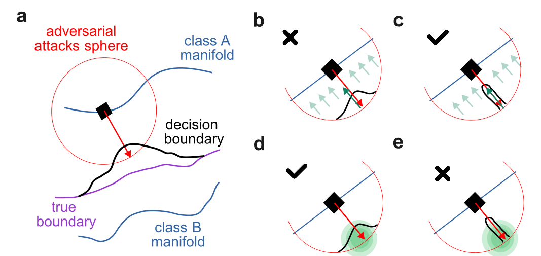
Why combining both defenses makes sense. Filters and noise are complementary by design. Filters suppress attacks that are far from the image manifold, but miss attacks that hug it closely. Noise disrupts thin filament-like attacks, but is powerless against large, compact adversarial blobs. Together, they cover a wider range of attack geometries than either method alone. In practice, we recommend applying noise first and then filtering, since this ordering preserves clean accuracy better. It is also worth noting that adversarial training---which pushes the learned decision boundary toward the true human boundary---directly reduces $V_a(x)$, making it a natural complement to both defenses, albeit at significant training cost.
2 - Experiments
We start with an ablation on CIFAR10 under standard and adversarial evaluation. The key result is that noise and bilateral filtering are complementary: each method improves robustness in different attack regimes, while their combination gives the strongest overall gains.
| Method | Clean | FGSM | L∞ | EoT. | L2 | C&W |
|---|---|---|---|---|---|---|
| Standard CNN | 74.5% ±2.4 | 3.5% ±2.1 | 0.2% ±0.4 | 0.2% ±0.5 | 1.3% ±0.6 | 0.6% ±0.6 |
| + Bil. | 69.0% ±2.2 | 10.0% ±1.2 | 1.0% ±0.4 | 1.2% ±0.5 | 11.9% ±1.4 | 0.5% ±0.3 |
| + Noise | 68.5% ±1.7 | 22.8% ±1.3 | 25.5% ±1.2 | 12.0% ±0.9 | 49.6% ±1.4 | 43.0% ±1.0 |
| + Noise + Bil. | 67.9% ±1.4 | 33.9% ±1.7 | 36.5% ±1.5 | 18.9% ±1.4 | 58.5% ±1.7 | 47.2% ±1.0 |
| + Bil. + Noise | 67.5% ±0.3 | 30.8% ±0.5 | 28.1% ±0.5 | 15.1% ±0.5 | 54.1% ±0.4 | 41.8% ±0.6 |
| Linear gain | -11.5% | 25.8% | 26.1% | 12.8% | 58.9% | 42.3% |
| Actual gain | -6.6% | 30.4% | 36.2% | 18.7% | 57.2% | 46.6% |
| Method | Epochs | Artificial data | Clean | AutoAttack | EoT AutoAttack |
|---|---|---|---|---|---|
| WRN-28-4 | 400 | 1 M | 87.44% | 58.28% | - |
| + Prepro. 10/50 | 86.32% | 67.24% | 62.36% | ||
| WRN-28-10 | 400 | 1 M | 88.96% | 61.60% | - |
| + Prepro. 10/50 | 87.70% | 68.56% | 63.68% | ||
| + Prepro. 20/80 | 88.24% | 69.60% | 67.2% | ||
| WRN-28-10 | 2400 | 20 M | 90.12% | 64.40% | - |
| + Prepro. 20/80 | 90.52% | 73.08% | 70.9% | ||
| SotA model | 10000 | 500 M | 93.68% | 73.71% | - |
| WRN-82-12 | 3000 | 150 M | 93.04% | 71.41% | - |
| + Prepro. 20/100 | 3000 | 50 M | 90.12% | 74.32% | 73.00% |
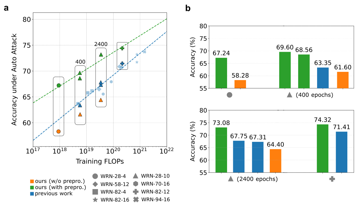
Test accuracy (%) under AutoAttack as a function of training FLOPs. Models trained with the preprocessor are shown in green, models without it in orange, and previous work in blue. The preprocessor improves robust accuracy at similar training cost and matches stronger baselines that require substantially more compute. Panel (b) compares selected model families from panel (a), highlighting the gains from preprocessing at 400 and 2400 training epochs.
3 - Discussion
In this work, we analyzed how idealized denoising filters and Gaussian noise affect the geometry of adversarial attacks. The main takeaway is that the two methods cancel different attack shapes: filters suppress perturbations far from the image manifold, while noise disrupts thin, localized adversarial regions. This complementarity motivates combining them.
Experimentally, a preprocessor that combines Gaussian noise with bilateral filtering gives supra-linear gains in adversarial robustness compared to either method alone, while keeping the drop in clean accuracy small. When combined with adversarially trained WRNs, the same idea improves robustness across the attacks we tested, including AutoAttack and attacks designed to target the preprocessor directly.
The result is a lightweight way to improve robustness with minimal computational overhead. For the full mathematical analysis, attack setup, and extended benchmarks, see the CVPR 2026 paper.
refs:
[1] Synthesizing Robust Adversarial Examples. Athalye, A., Engstrom, L., Ilyas, A., and Kwok, K. In Proceedings of the 35th International Conference on Machine Learning, pages 284-293. PMLR, 2018.
[2] Intriguing Properties of Neural Networks. Szegedy, C., Zaremba, W., Sutskever, I., Bruna, J., Erhan, D., Goodfellow, I., and Fergus, R. arXiv:1312.6199, 2014.
[3] RobustBench: A Standardized Adversarial Robustness Benchmark. Croce, F., Andriushchenko, M., Sehwag, V., Debenedetti, E., Flammarion, N., Chiang, M., Mittal, P., and Hein, M. arXiv:2010.09670, 2020.